From an agent-centric point of view, what is “near” but what is easy to achieve; what is “far” but what is difficult to approach? At any moment, we take stock of what actions we can perform and their consequences for us, and struggle our way to some destination which is not so much a physical place as the redemption of a goal, the fulfillment of a dream. We would like to regard space and time as ways of organizing ourselves in relation to our goals. How can we cash this idea out? In the 1930’s, Walter Lewin introduced the idea of hodological space from the Greek word hodos meaning path [1]. The hodological space of an agent is the space of their possible movement, shaped by their capabilities and their goals. Our question: under what circumstances can we in fact identify the hodological space of an agent with the usual notion of space? We give here a simple toy example.

1. Background on Bellman

Let us consider a finite Markov decision process. In this type of model, at time \(t\) the agent observes one of a finite number of states \(S_t=s\), selects one of a finite number of actions \(A_t=a\), and the environment samples the next state according to \[\tag{1.1}\begin{aligned}P(s^\prime|s, a) \equiv P(S_{t+1}=s^\prime| S_t=s, A_t=a).\end{aligned}\]

The agent then receives an immediate reward \(R_{t+1}\). Let \(0\leq \gamma \leq 1\) be the temporal discount factor. For a problem with an infinite temporal horizon, the discounted reward from time \(t\) onward is \[\tag{1.2}\begin{aligned}G_t = \sum_{k=0}^\infty \gamma^k R_{t+k+1}.\end{aligned}\]

In contrast, for a problem which terminates when a goal is reached, the sum becomes finite. A policy \(\pi(a|s) \equiv P(A_t=a|S_t=s)\) is a distribution over possible actions conditional on the current state: the agent will sample from this distribution to choose its next action. Given a policy \(\pi\), let \[\tag{1.3}\begin{aligned}Q^{\pi}(s,a) = \mathbb{E}^\pi \left[ G_t | S_t=s, A_t=a\right]\end{aligned}\]

be the expected total future return conditional on first choosing \(a\) in state \(s\), and then following policy \(\pi\). Denote the optimal state/action value by \[\tag{1.4}\begin{aligned}Q^*(s,a) = \sup_\pi Q^\pi(s,a):\end{aligned}\]

it is the expected total future return conditional on first choosing \(a\) in state \(s\), and then acting optimally afterwards. Finally, denote the optimal state value by \[\tag{1.5}\begin{aligned}V^*(s) = \max_a Q^*(s,a).\end{aligned}\]

If the immediate reward is \(R(s,a)\), the Bellman optimality equation [2, 3] is \[\tag{1.6}\begin{aligned}Q^*(s,a) &= R(s,a) + \gamma \sum_{s^\prime} P(s^\prime|s, a)V^*(s^\prime)\end{aligned}\]

or equivalently, \[\tag{1.7}\begin{aligned}V^*(s) = \max_a \left[R(s,a) + \gamma \sum_{s^\prime} P(s^\prime|s, a) V^*(s^\prime)\right].\end{aligned}\]

We can view this equation as a constraint on the optimal values \(V^*(s)\). (Note that more generally, one can consider nondeterministic rewards, in which case the average should be taken over possible rewards as well.)

A special case of a Markov decision process is a stochastic shortest path problem. Suppose we fix a goal state \(g\) and suppose that an episode for the agent terminates upon reaching the goal. The agent is interested in getting to the goal as quickly as possible. To formalize this, we assume that every selected action has reward \(-1\), and we assume no temporal discounting: \(\gamma=1\). Let \(V^*_g(s)\) be the value of \(s\) when the goal is \(g\). If the agent reaches the goal state, the episode is over—no action is taken and no reward received. Thus \[\tag{1.8}\begin{aligned}V_g^*(g)= 0.\end{aligned}\]

Otherwise, if \(s\neq g\), we have \[\tag{1.9}\begin{aligned}Q_g^*(s,a) = -1 + \sum_{s^\prime} P(s^\prime|s,a)V_g^*(s^\prime) && V_g^*(s) = \max_a Q_g^*(s,a).\end{aligned}\]

Alternatively, we can express the optimality equation in terms of the optimal expected number of steps (the cost) required to reach the goal \(g\) from state \(s\), \[\tag{1.10}\begin{aligned}C^*_g(s) = -V_g^*(s) = \min_a C^*_g(s,a),\end{aligned}\]

where \(C^*_g(s,a) = - Q_g^*(s,a)\) is the optimal cost given that the agent first chose action \(a\). In particular \(C^*_g(g)=0\), and \[\tag{1.11}\begin{aligned}C^*_g(s,a) = 1 + \sum_{s^\prime} P(s^\prime|s, a)C^*_g(s^\prime).\end{aligned}\]

We would like to regard \(C^*_g(s)\) as the distance between the state \(s\) and the goal \(g\) in hodological space. We now turn to a simple example where points in this hodological space can in fact be identified with points in ordinary Euclidean space.

2. A toy example

Let there be four possible states \(s\in \{0,1,2,3\}\) and three possible actions \(a \in \{0, 1, 2\}\). The goal is to end up in a particular state \(g\), and we are interested in getting there as quickly as possible: as above, we assume that every selected action has reward \(-1\), and we assume no temporal discounting: \(\gamma=1\). The response of the environment is encoded in \(P(s^\prime|s, a)\), which we take to be \[\tag{2.1}\begin{aligned}P(s^\prime|s, 0) = \begin{pmatrix} 0 & 1 & 0 & 0 \\ 1 & 0 & 0 & 0 \\ 0 & 0 & 0 & 1 \\ 0 & 0 & 1 & 0 \end{pmatrix} && P(s^\prime|s, 1) = \begin{pmatrix} 0 & 0 & 1 & 0 \\ 0 & 0 & 0 & 1 \\ 1 & 0 & 0 & 0 \\ 0 & 1 & 0 & 0 \end{pmatrix},\end{aligned}\]

and letting \(p = 1/\sqrt{2}\), \[\tag{2.2}\begin{aligned}P(s^\prime|s, 2) = \begin{pmatrix} 1-p & 0 & 0 & p \\ 0 & 1-p & p & 0 \\ 0 & p & 1-p & 0 \\ p & 0 & 0 & 1-p \end{pmatrix} .\end{aligned}\]

In other words, choosing action \(a=0\) swaps states \(0\leftrightarrow 1\) and \(2 \leftrightarrow 3\); choosing action \(a=1\) swaps states \(0 \leftrightarrow 2\) and \(1 \leftrightarrow 3\); and finally, choosing action \(a=2\) swaps \(0\leftrightarrow 3\) and \(1 \leftrightarrow 2\) with probability \(p\) (success), but with probability \(1-p\) does nothing (failure).

For this setup, we can calculate the optimal cost values \(C_g^*(s)\) explicitly. Suppose \(g=0\). Immediately, we have \(C_0^*(0)=0\). Moreover, if \(g=0\) and \(s=1\) and the agent chooses \(a=0\), then since \(P(s^\prime =0|s=1,a=0)=1\), the agent moves deterministically to the goal state. From \[\tag{2.3}\begin{aligned}C^*_g(s,a) = 1 + \sum_{s^\prime} P(s^\prime|s, a)C^*_g(s^\prime),\end{aligned}\]

we conclude \[\tag{2.4}\begin{aligned}C_0^*(1,0) = 1 + \sum_{s^\prime} P(s^\prime|1,0)C^*_0(s^\prime) = 1 + C_0^*(0) = 1.\end{aligned}\]

Starting from \(s=1\), clearly at least one action must be taken to reach the goal \(g=0\): thus \(C_0^*(1) \geq 1\). The above achieves this lower bound, and so \(C_0^*(1) = 1\). Similarly, action \(a=1\) moves deterministically from \(s=2\) to the goal \(g=0\) since \(P(s^\prime=0|s=2,a=1)=1\). We conclude \[\tag{2.5}\begin{aligned}C_0^*(2,1) = 1 + C_0^*(0) = 1.\end{aligned}\]

By the same argument \(C_0^*(2)=1\). Finally, we must calculate \(C_0^*(3)\). This one is a little more interesting. Action \(a=0\) sends \(3 \rightarrow 2\) and \(a=1\) sends \(3 \rightarrow 1\) in both cases deterministically. Therefore \[\tag{2.6}\begin{aligned}C_0^*(3,0) = 1 + C_0^*(2) = 2 && C_0^*(3,1)=1+C_0^*(1) = 2.\end{aligned}\]

On the other hand, \(a=2\) takes the state from \(3 \rightarrow 0\) with probability \(p\), but leaves the state at \(3\) with probability \(1-p\) so that \[\tag{2.7}\begin{aligned}C_0^*(3,2) &= 1 + pC_0^*(0) + (1-p)C_0^*(3) = 1 + (1-p)C_0^*(3).\end{aligned}\]

After an “unsuccessful” outcome, the agent remains at 3: in this case, the agent is free to choose the optimal action again whatever that may be. Thus \[\tag{2.8}\begin{aligned}C_0^*(3) = \min_a C_0^*(3,a) = \min \left\{ 2,2, 1 + (1-p)C_0^*(3)\right\}.\end{aligned}\]

Suppose action \(a=2\) were optimal. Then \(C_0^*(3) = 1 + (1-p)C_0^*(3)\) which implies \(C_0^*(3)=1/p = \sqrt{2}\). Since \(\sqrt{2} < 2\), this indeed gives the optimal value: the single action \(a=2\) is better than either two-step deterministic route (choosing \(a=1\) and then \(a=2\), or \(a=2\) and then \(a=1\)). Moreover, the value of \(\sqrt{2}\) can be interpreted as the expected number of attempts (at choosing \(a=2\)) required to obtain a successful outcome. Indeed, let \(N\) be the number of attempts to move from \(3\rightarrow 0\). Then \[\tag{2.9}\begin{aligned}P(N = n) = (1-p)^{n-1} p,\end{aligned}\]

so that \[\tag{2.10}\begin{aligned}\mathbb{E}[N] &= \sum_{n=0}^\infty n (1-p)^{n-1} p = p \frac{d}{dx} \sum_{n=0}^\infty x^n = p \frac{d}{dx} \frac{1}{1-x}= \frac{1}{p},\end{aligned}\]

where we set \(x=1-p\) and used the fact that the sum of a geometric series for \(|x|< 1\) is \(\sum_{n=0}^\infty x^n = 1/(1-x)\). We conclude that \(\mathbb{E}[N] = 1/p = \sqrt{2}\).

Putting it all together, we find \[\tag{2.11}\begin{aligned}\begin{pmatrix} C_0^*(0)\\ C_0^*(1)\\ C_0^*(2)\\ C_0^*(3) \end{pmatrix} = \begin{pmatrix} 0\\ 1\\ 1\\ \sqrt{2} \end{pmatrix}.\end{aligned}\]

One may repeat precisely the same arguments for the other goals \(g=1,2,3\). In fact, the situation is completely symmetrical, which leads to an overall cost matrix \[\tag{2.12}\begin{aligned}C^* = [C_g^*(s)]_{g,s} = \begin{pmatrix} 0 & 1 & 1 & \sqrt{2}\\ 1 & 0 & \sqrt{2} & 1\\ 1 & \sqrt{2} & 0 & 1\\ \sqrt{2} & 1 & 1 & 0 \end{pmatrix}.\end{aligned}\]

In fact, this is the Euclidean distance matrix of the four vertices of a unit square in 2D. For example, one may check that if \[\tag{2.13}\begin{aligned}x_0= \begin{pmatrix}0\\0\end{pmatrix}, \qquad x_1= \begin{pmatrix}1\\0\end{pmatrix}, \qquad x_2= \begin{pmatrix}0\\1\end{pmatrix}, \qquad x_3= \begin{pmatrix}1\\1\end{pmatrix},\end{aligned}\]

we have \[\tag{2.14}\begin{aligned}C_g^*(s) = \lVert x_s - x_g \rVert_2.\end{aligned}\]

We conclude that the optimal cost of getting from \(s\rightarrow g\) can be interpreted as the geometric distance between two points on the unit square: the hodological space of the agent can be identified with this lattice of points in two dimensional Euclidean space.

Keeping the states and transitions fixed, simply by changing the nature of the actions avaliable to the agent, the hodological space will be different. For instance, suppose \(a=3\) simply swapped \(0\leftrightarrow 3\) and \(1 \leftrightarrow 2\) deterministically. Then \[\tag{2.15}\begin{aligned}C^* = \begin{pmatrix} 0 & 1 & 1 & 1\\ 1 & 0 &1 & 1\\ 1 & 1 & 0 & 1\\ 1 & 1 & 1 & 0 \end{pmatrix},\end{aligned}\]

which corresponds to the distance matrix of a regular tetrahedron in 3D with unit edge lengths, e.g., \[\tag{2.16}\begin{aligned}x_0 = \frac{1}{2\sqrt{2}} \begin{pmatrix} 1\\ 1\\ 1 \end{pmatrix}, \qquad x_1 = \frac{1}{2\sqrt{2}} \begin{pmatrix} 1\\ -1\\ -1 \end{pmatrix},\end{aligned}\]

\[\begin{aligned} x_2 = \frac{1}{2\sqrt{2}} \begin{pmatrix} -1\\ 1\\ -1 \end{pmatrix}, \qquad x_3 = \frac{1}{2\sqrt{2}} \begin{pmatrix} -1\\ -1\\ 1 \end{pmatrix}.\end{aligned}\] More generally, however, \(C^*\) may not be interpretable as the distance matrix of points in any Euclidean space. Notice that in our example, we have \(C^*_s(s^\prime) = C^*_{s^\prime}(s)\): if this symmetry is violated, a Euclidean interpretation is already off the table.

3. Schoenberg

Suppose we have a matrix \(\Delta_{ij}\) of purported distances between points \(\{x_i\}\). How can we check if there really does exist such a set of points in some dimension \(d\) corresponding to \(\Delta_{ij}\)?

Let \(\{x_i\}_{i=1}^n\) be a set of real vectors in \(d\)-dimensional space, and let \(G_{ij} = x_i \cdot x_j\) be its Gram matrix. Recall that \(G=G^T\) is a Gram matrix of real vectors iff \(G \ge 0\), that is, \(G\) is positive semidefinite. To see this, note that on the one hand, if \(G\) is a Gram matrix, then \[\tag{3.1}\begin{aligned}\forall c \in \mathbb{R}^n: c^T G c = \sum_{ij} c_i c_j x_i \cdot x_j = \lVert \sum_i c_i x_i \rVert^2 \ge 0\end{aligned}\]

shows that \(G\) is positive semidefinite. On the other hand, if \(G \ge 0\), by the spectral decomposition \(G=Q\Lambda Q^T\), we can express \(G=XX^T\) where the rows of \(X=Q\sqrt{\Lambda}\) are (not uniquely) the corresponding vectors \(\{x_i\}\). In other words, given a symmetric matrix \(G\) of purported inner products, we can check whether a set of vectors \(\{x_i\}\) exists which realizes \(G\): we simply check whether \(G\) is positive semidefinite, and then we can reconstruct \(\{x_i\}\) up to overall rotations. We would therefore like to convert our problem of reconstructing points from distances to the problem of reconstructing vectors from inner products.

To this end, notice that the squared distances \(\Delta^{2}_{ij}\) between the vectors \(\{x_i\}\) can be expressed \[\tag{3.2}\begin{aligned}\Delta^{2}_{ij} = \lVert x_i - x_j \rVert^2 &= (x_i - x_j) \cdot (x_i - x_j)\end{aligned}\] \[\tag{3.3}\begin{aligned}&= \lVert x_i \rVert^2 + \lVert x_j \rVert^2 - 2x_i \cdot x_j\end{aligned}\] \[\tag{3.4}\begin{aligned}&= G_{ii} + G_{jj} - 2 G_{ij},\end{aligned}\]

or \(\Delta^{\circ 2} = g u^T + u g^T - 2 G\), where \(u = (1,\dots,1)^T\) and \(g = (G_{11}, \dots, G_{nn})^T\). In this way, we can express the distance matrix \(\Delta\) in terms of the Gram matrix \(G\). But whereas distances are invariant under collective translations of the vectors, \(\lVert (x_i + a) - (x_j +a)\rVert = \lVert x_i - x_j\rVert\), the Gram matrix is not: \((x_i + a) \cdot (x_j + a) \neq x_i \cdot x_j\). To get a unique Gram matrix which allows us to reconstruct points from distances, we must make a choice of the origin: we assume in particular that the centroid of all the points \(\{x_i\}\) is at the origin: \(\sum_i x_i = 0\). Let \(\Pi_0 = I - J/n\) where \(J\) is the matrix of all 1’s: this projects onto the subspace of vectors orthogonal to \(u\), that is, the subspace of vectors summing to 0. Then \[\tag{3.5}\begin{aligned}\Pi_0 \Delta \Pi_0 = \Pi_0(g u^T + u g^T - 2 G)\Pi_0 = -2 \Pi_0 G \Pi_0 = -2 G,\end{aligned}\]

where the last follows from the assumption that the vectors are centered: \(G u = \sum_{j} x_i \cdot x_j = x_i \cdot \sum_j x_j=0\). We conclude that for centered vectors, \(G = -\frac{1}{2}\Pi_0 \Delta \Pi_0\).

So: given a set of vectors \(\{x_i\}\) whose centroid is zero, their Gram matrix can be expressed \(G = -\frac{1}{2}\Pi_0 \Delta^{\circ 2} \Pi_0 \ge 0\) where \(\Pi_0\) projects onto the zero-sum subspace and \(\Delta\) is the matrix of distances between the points. In particular, \(\Delta\) must be symmetric and have zeros along its diagonal. Conversely, given \(\Delta=\Delta^T\) with zeros along its diagonal, suppose \(G = -\frac{1}{2}\Pi_0 \Delta^{\circ 2} \Pi_0 \ge 0\). By the spectral decomposition, we can write \(G= X X^T\), letting \(\{x_i\}\) be the rows of \(X\). We have \[\tag{3.6}\begin{aligned}\lVert x_i - x_j \rVert^2 = G_{ii} + G_{jj} - 2 G_{ij} = (e_i - e_j)^T G (e_i - e_j) = z^T G z,\end{aligned}\]

where \(z = e_i - e_j\) for basis vectors \(\{e_i\}\). Clearly \(u^T z = 0\) and \(Jz = z\). But from the definition of \(G\), \[\tag{3.7}\begin{aligned}\lVert x_i - x_j \rVert^2 &= z^T \left[-\frac{1}{2}\Pi_0 \Delta^{\circ 2} \Pi_0\right] z = -\frac{1}{2} z^T \Delta^{\circ 2} z\end{aligned}\] \[\tag{3.8}\begin{aligned}&= \Delta^{\circ 2}_{ii} - \Delta^{\circ 2}_{ij} - \Delta^{\circ 2}_{ji} + \Delta^{\circ 2}_{jj} = - \frac{1}{2}\Delta^{\circ 2}_{ij},\end{aligned}\]

as desired, where we have used both the symmetry of \(\Delta\) and the fact that its diagonal is 0. This completes the proof.

Theorem 3.1. (Schoenberg [7])

Let \(\Delta\in \mathbb{R}^{n \times n}\) satisfy \(\Delta=\Delta^T\) and \(\forall i: \Delta_{ii} = 0\). Then \(\Delta\) can be realized as the matrix of Euclidean distances \(\Delta_{ij} = \lVert x_i - x_j\rVert\) for vectors \(\{x_i\}\) (which without loss of generality satisfy \(\sum_i x_i = 0\)) iff \[\tag{3.9}\begin{aligned}G= -\frac{1}{2}\Pi_0 \Delta^{\circ 2} \Pi_0 \ge 0,\end{aligned}\]

where \(\Pi_0 = I - J/n\).

Corollary 3.2.

Schoenberg’s condition is often equivalently expressed: \(\Delta=\Delta^T\) with \(\Delta_{ii}=0\) is a matrix of distances iff \(\forall u^Tz = 0: z^T \Delta^{\circ 2} z \leq 0\).

Corollary 3.3.

The construction suggests a measure of how far \(\Delta\) is from a distance matrix. Use the eigendecomposition to separate \(G = G_+ - G_-\) into the difference of two PSD matrices. Then \[\tag{3.10}\begin{aligned}\mathcal{E}(\Delta) = \frac{\lVert G_- \rVert_F}{\lVert G \rVert_F}\end{aligned}\]

will be zero iff \(G \ge 0\).

Corollary 3.4.

Finally, the same construction tells us the minimum dimension required for a set of points \(\{x_i\}\) to realize the required distances. Indeed, it is just \(d=\text{rank}(G)\). We can reconstruct the \(d\)-dimensional vectors from the spectral decomposition \[\tag{3.11}\begin{aligned}G = Q \Lambda Q^T = \begin{pmatrix} A & B \\ C & D \end{pmatrix} \begin{pmatrix} \Lambda_d & 0 \\ 0 & 0 \end{pmatrix} \begin{pmatrix} A^T & C^T \\ B^T & D^T \end{pmatrix} = \begin{pmatrix} A \sqrt{\Lambda_d} & C \sqrt{\Lambda_d} \end{pmatrix} \begin{pmatrix} \sqrt{\Lambda_d}A^T \\ \sqrt{\Lambda_d}C^T \end{pmatrix} = X X^T,\end{aligned}\]

where \(X \in \mathbb{R}^{n \times d}\).

4. Possible geometries

Considering again our toy model, let us consider arbitrary values of \(p\), the success probability for action \(a=3\). For \(p\ge 1/2\), the optimal cost matrix is then \[\tag{4.1}\begin{aligned}C^* = \begin{pmatrix} 0 & 1 & 1 & 1/p\\ 1 & 0 & 1/p & 1\\ 1 & 1/p & 0 & 1\\ 1/p & 1 & 1 & 0 \end{pmatrix}.\end{aligned}\]

Let \(\Delta \equiv C^*\). The eigenvalues of \(G = -\frac{1}{2}\Pi_0 \Delta^{\circ 2} \Pi_0\) can be explicitly calculated: \[\tag{4.2}\begin{aligned}\lambda \in \left\{0, \frac{1}{2p^2}, \frac{1}{2p^2}, 1- \frac{1}{2p^2}\right\}.\end{aligned}\]

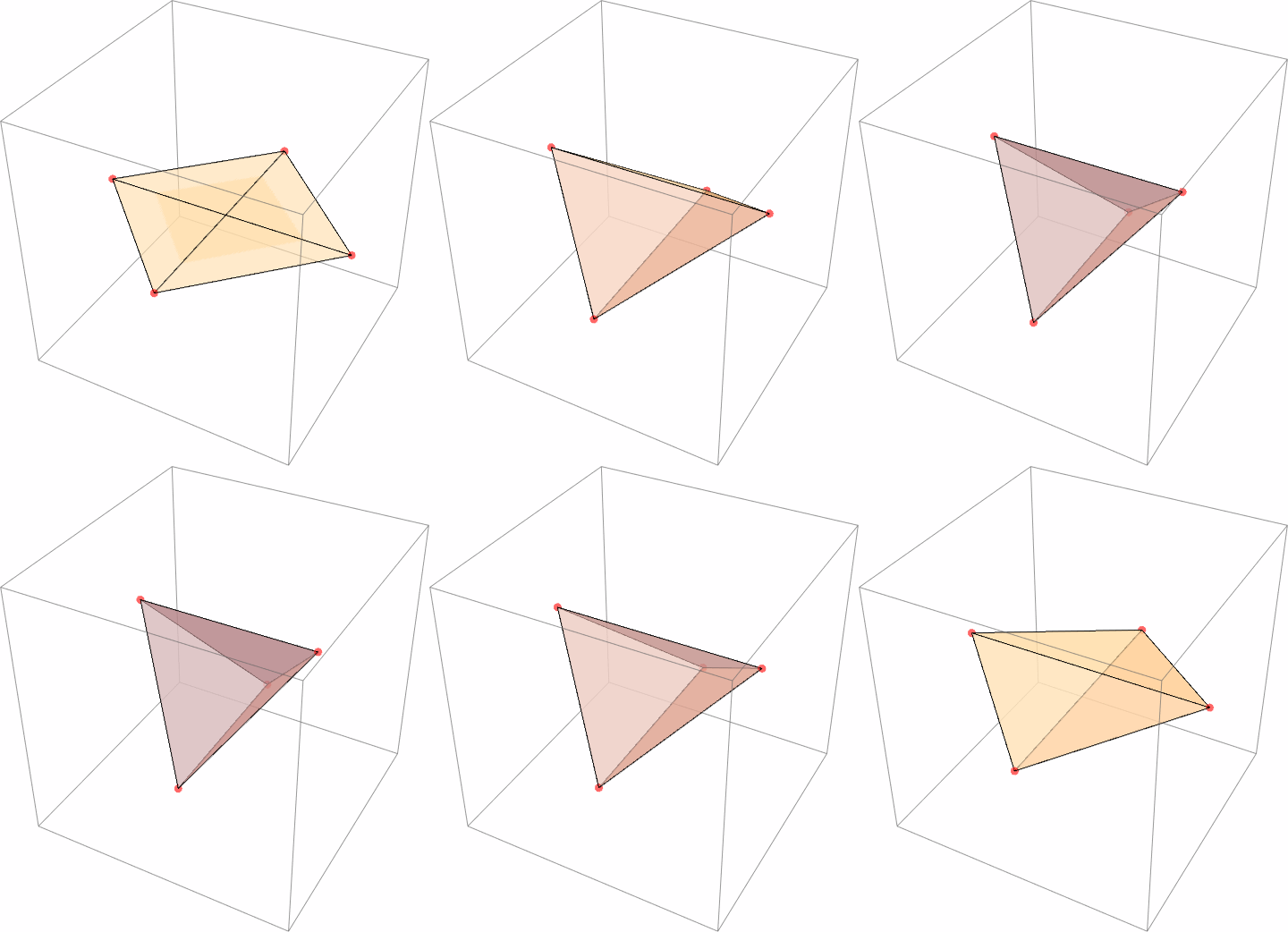
Since \(p>0\), we conclude that the cost matrix can be realized as a matrix of Euclidean distances iff \(p \ge 1/\sqrt{2}\). We can therefore explore the geometries associated with each value of \(p\) in the interval \[\tag{4.3}\begin{aligned}\frac{1}{\sqrt{2}} \leq p \leq 1.\end{aligned}\]

When \(p = 1/\sqrt{2}\), the final eigenvalue vanishes, and we have the two dimensional realization as a square. When \(p=1\), we have the three dimensional realization as a regular tetrahedron. In between we have nonregular tetrahedra interpolating between them.

But this is only half the story. The triangle inequality is a defining property of any norm: it requires that \(\lVert u + v \rVert \leq \lVert u \rVert + \lVert v \rVert\). In fact, \(d(x,z) \leq d(x,y) + d(y,z)\) on any three points on a Riemannian manifold. From the form of \(C^*\), any three of the purported vertices form a triangle with side lengths \(1, 1\), and \(1/p\). By the triangle inequality, therefore, \(1/p \leq 2\), or \(p \ge 1/2\) which is a looser bound than \(p\ge 1/\sqrt{2}\). In fact, in our original derivation, we showed that \(C_0^*(3) = \min\{2, 1/p\}\) which guarantees the triangle inequality will be satifies in our model. But we have just shown that for \(1/2 \leq p < 1/\sqrt{2}\), there is no Euclidean realization. But what about a non-Euclidean realization?

Recall that the Gaussian curvature \(K\) is a scalar measure of how a surface curves at some point. If \(K>0\), the surface curves like a sphere; if \(K=0\), the surface is flat in at least one direction; if \(K<0\), the surface curves like a saddle. In particular, let us consider a sphere of radius \(R\). For two points on the sphere, we have \(x_i \cdot x_j = \lVert x_i \rVert \lVert x_j \rVert \cos \theta_{ij} = R^2 \cos \theta_{ij}\) where \(\theta_{ij}\) is the angle between them. At the same time, the shortest path on a sphere between two points—a geodesic—is a great circle arc, where the arclength is defined as \(\Delta_{ij} = R\theta_{ij}\). Finally, a sphere of radius \(R\) has constant Gaussian curvature \(K=1/R^2\). We conclude \[\tag{4.4}\begin{aligned}x_i \cdot x_j = K^{-1} \cos(\sqrt{K}\Delta_{ij}).\end{aligned}\]

Let us therefore consider the Gram matrix \(G= K^{-1} \cos(\sqrt{K} C^*_{ij})\), or \[\tag{4.5}\begin{aligned}G = K^{-1}\begin{pmatrix} 1 & r & r & t\\ r & 1 & t & r\\ r & t & 1 & r\\ t & r & r & 1 \end{pmatrix} && r = \cos(\sqrt{K}) && t = \cos(\sqrt{K}/p).\end{aligned}\]

The eigenvalues of this matrix are \[\tag{4.6}\begin{aligned}\lambda \in \left\{ 1 - \cos(\sqrt{K}/p), 1 - \cos(\sqrt{K}/p), 1 - 2 \cos(\sqrt{K}) + \cos(\sqrt{K}/p), 1 + 2 \cos(\sqrt{K}) + \cos(\sqrt{K}/p)\right\}.\end{aligned}\]

If we want a realization on the 2-sphere in three dimensions, we require \(G\) to have rank 3. From the form of the eigenvalues, this forces \[\tag{4.7}\begin{aligned}1 - 2 \cos(\sqrt{K}) + \cos(\sqrt{K}/p) = 0,\end{aligned}\]

which relates the curvature \(K\) to the success probability \(p\). Suppose \(p = 1/2\). Since \(K>0\), this forces \(K = \pi^2/4\). We can therefore realize the required distances as points on a 2-sphere of radius \(R=2/\pi\). Below we plot on the one hand, the Gaussian curvature \(K\) as a function of \(p\), and on the other hand, the radius \(R\) of the sphere as a function of \(p\). As \(p\rightarrow 1/\sqrt{2}\), the radius diverges, and we recover the flat space case.

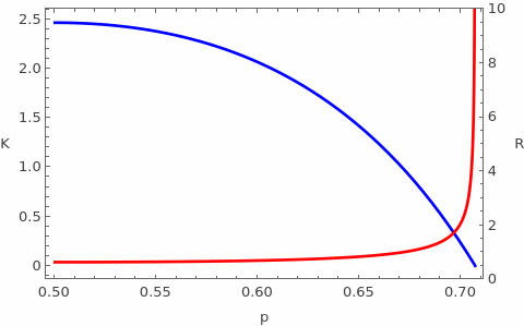
Thus for \(0 \leq p < 1/\sqrt{2}\), we have a realization on the surface of a 2-sphere—in fact, for \(0 \leq p \leq 1/2\) each realization is the same, on a sphere with radius \(R = 2/\pi\); for \(p= 1/\sqrt{2}\), we have a realization in 2D Euclidean space; and for \(1/\sqrt{2} < p \leq 1\), we have a realization in 3D Euclidean space.

5. \(Q\)-learning

So far we have been able to analyze our decision process analytically. In practice, however, one uses a reinforcement learning algorithm to train an agent to navigate its environment. Let us see how that might work in the simplest possible case.

As we’ve seen, the Bellman optimality equation is \[\begin{aligned} Q^*(s,a) &= R(s,a) + \gamma \sum_{s^\prime} P(s^\prime|s, a)V^*(s^\prime).\end{aligned}\] But since \(V^*(s) = \max_a Q^*(s,a)\), this amounts to \[\begin{aligned} Q^*(s,a) &= R(s,a) + \gamma \sum_{s^\prime} P(s^\prime|s, a)\max_{a^\prime} Q^*(s,a^\prime).\end{aligned}\] Suppose we have a candidate \(Q\)-function \(Q(s,a)\). Let \(T\) be the Bellman operator, which acts on \(Q\)-functions as \[\tag{5.1}\begin{aligned}(TQ)(s,a) &= R(s,a) + \gamma \sum_{s^\prime} P(s^\prime|s, a)\max_{a^\prime} Q(s,a^\prime).\end{aligned}\]

In other words, \(TQ\) is a \(Q\)-function which gives the expected total future return conditional on first choosing \(a\) in state \(s\), and then acting optimally according to \(Q(s,a)\) afterwards. In particular, the optimal \(Q\)-function satisfies \(Q^*= T Q^*\): it is a fixed point of the Bellman operator. Now suppose \(Q_1\) and \(Q_2\) are two different \(Q\)-functions, and we consider their difference \[\tag{5.2}\begin{aligned}(TQ_1)(s,a) - (TQ_2)(s,a) &= \gamma \sum_{s^\prime} P(s^\prime|s, a)\Big(\max_{a^\prime} Q_1(s,a^\prime) - \max_{a^\prime} Q_2(s, a^\prime)\Big)\end{aligned}\] \[\tag{5.3}\begin{aligned}&= \gamma \mathbb{E}[\max_{a^\prime} Q_1(s,a^\prime) - \max_{a^\prime} Q_2(s, a^\prime)].\end{aligned}\]

But \[\tag{5.4}\begin{aligned}\Big|\max_{a} Q_1(s,a) - \max_{a} Q_2(s, a)\Big| \leq \max_{a} \Big|Q_1(s, a)- Q_2(s, a)\Big|,\end{aligned}\]

and so letting \[\tag{5.5}\begin{aligned}\lVert Q_1 - Q_2 \rVert_\infty = \max_{s,a}|Q_1(s,a) - Q_2(s,a)|,\end{aligned}\]

we have \[\tag{5.6}\begin{aligned}\lVert TQ_1 - TQ_2 \rVert_\infty \leq \gamma \lVert Q_1 - Q_2 \rVert_\infty.\end{aligned}\]

From this we see that the Bellman operator acts as a contraction. Now let \(Q_n = T^n Q\). Chaining inequalities and recalling that \(Q^*\) is a fixed point of \(T\), we have for example \[\tag{5.7}\begin{aligned}\lVert Q_2 - Q^* \rVert_\infty \leq \gamma \lVert Q_1 - Q^* \rVert_\infty \leq \gamma^2 \lVert Q_0 - Q^* \rVert_\infty,\end{aligned}\]

and in general, \[\tag{5.8}\begin{aligned}\lVert Q_n - Q^* \rVert \leq \gamma^n \lVert Q_0 - Q^*\rVert_\infty.\end{aligned}\]

Since \(\gamma^n \rightarrow 0\), by iterating the Bellman operator, \(Q_n \rightarrow Q^*\). In other words, no matter which \(Q\)-function we start with, by repeated application of the Bellman operator we can approach the optimal \(Q\)-function.

This is nice, but to evaluate the action of the Bellman operator we need the conditional probabilities \(P(s^\prime|s, a)\) for a transition to a future state \(s^\prime\) given a previous state \(s\) and action \(a\). But what if the agent knows nothing of probabilities? Instead, the agent could start with an initial \(Q\)-function \(Q(s,a)\) with all values initialized to zero. Upon taking an action \(a\) and transitioning from \(s\) to \(s^\prime\) while receiving reward \(r\), the agent can compute \[\tag{5.9}\begin{aligned}Y = r + \gamma \max_{a^\prime} Q(s^\prime, a^\prime).\end{aligned}\]

Notice that \[\tag{5.10}\begin{aligned}\mathbb{E}[Y|s,a] = r + \sum_{s^\prime} P(s^\prime|s, a)\max_{a^\prime}Q(s^\prime, a^\prime) = (TQ)(s,a).\end{aligned}\]

In other words, \(Y\) is a random variable whose average is the Bellman updated \(Q\)-function. Therefore instead of calculating \(TQ\) directly, which requires probability assignments \(P(s^\prime|s, a)\), the agent can use the random sample to nudge its current \(Q\) function in the right direction. If \(Q_t(s,a)\) is the \(Q\)-function at time \(t\), then the agent updates \[\tag{5.11}\begin{aligned}Q_{t+1}(s,a) = (1-\alpha_t)Q_t(s,a) + \alpha_t Y_t,\end{aligned}\]

where \(\alpha_t\) is some mixing parameter which ought to satisfy \(\sum_t \alpha_t = \infty\) so that learning never completely stops and \(\sum_t \alpha_t^2 < \infty\) to help with convergence: a common choice is \(\alpha_n = 1/n\) for the \(n\)th visit to \((s,a)\). Assuming that rewards are bounded, that \(0 \leq \gamma < 1\), that each state-action pair is visited infinitely often, and the above constraints on \(\alpha\), then one can show that eventually \(Q_t(s,a)\) will converge to \(Q^*(s,a)\) with probability 1.

This suggests a simple reinforcement learning algorithm [4]. The agent is armed with their \(Q\)-function, initialized to 0. At each time step, with some probability, an agent either takes a random action in hopes of exploring the territory, or else choses the action judged optimal by their \(Q\)-function given their current state \(s\). This is called an \(\epsilon\)-greedy strategy. Upon transitioning to state \(s^\prime\) and receiving reward \(r\), they update their \(Q\)-function using Eq. 5.11. Let \(\mathcal{S}\) be set of possible states and \(\mathcal{A}\) be the set of possible actions, and fix some discount factor \(0 \leq \gamma \leq 1\) and \(0 \leq \epsilon \leq 1\): for example, \(\epsilon = 0.1\).

Algorithm 1 Tabular Q-Learning

Initialize \(Q(s,a) \gets 0\) and \(n(s,a) \gets 0\) for all \(s \in \mathcal{S}\) and \(a \in \mathcal{A}\)
\(s \gets \class{algorithm-smallcaps}{\text{GetInitialState}}()\)
for \(t = 1,\ldots,T\) do
Draw \(u \sim \mathrm{Uniform}(0,1)\)
if \(u < \epsilon\) then
Choose \(a\) uniformly at random from \(\mathcal{A}\)
else
\(a \gets \arg\max_{a' \in \mathcal{A}} Q(s,a')\)
end if
\((s',r) \gets \class{algorithm-smallcaps}{\text{GetNextStateAndReward}}(s,a)\)
\(y \gets r + \gamma \max_{a' \in \mathcal{A}} Q(s',a')\)
\(n(s,a) \gets n(s,a) +1\)
\(\alpha \gets 1/n(s,a)\)
\(Q(s,a) \gets (1-\alpha)Q(s,a) + \alpha y\)
\(s \gets s'\)
end for

Now in the case of our toy model, we are interested in constructing an agent which keeps track of a \(Q\)-function for several different goals; whose experiences are organized into episodes which terminate upon reaching a prescribed goal; all of whose actions have reward \(-1\) to encourage them to learn the shortest path to each goal; and applies no temporal discounting. In other words:

Algorithm 2 Goal directed tabular Q-Learning

Initialize \(Q(s,a, g) \gets 0\) and \(n(s,a,g) \gets 0\) for all \(s \in \mathcal{S}\), \(a \in \mathcal{A}\), \(g \in \mathcal{S}\).
for episode \(= 1,\ldots,N\) do
\((s,g) \gets \class{algorithm-smallcaps}{\text{GetInitialStateAndGoal}}()\)
while \(s \neq g\) do
Draw \(u \sim \mathrm{Uniform}(0,1)\)
if \(u < \epsilon\) then
Choose \(a\) uniformly at random from \(\mathcal{A}\)
else
\(a \gets \arg\max_{a' \in \mathcal{A}} Q(s,a',g)\)
end if
\(s' \gets \class{algorithm-smallcaps}{\text{GetNextState}}(s,a)\)
if \(s' = g\) then
\(y \gets -1\)
else
\(y \gets -1 + \gamma \max_{a' \in \mathcal{A}} Q(s',a',g)\)
end if
\(n(s,a,g) \gets n(s,a,g) +1\)
\(\alpha \gets 1/n(s,a,g)\)
\(Q(s,a,g) \gets (1-\alpha)Q(s,a,g) + \alpha y\)
\(s \gets s'\)
end while
end for

Now in this case, there is no temporal discounting: thus the argument for convergence based on the contractive property of the Bellman operator does not apply. Instead, we can appeal to results of Tsitsiklis, Yu, and Bertsekas [5, 6]. Consider a finite stochastic shortest path problem with terminal state \(g\) which is absorbing (that is, the agent cannot leave it) and cost free after arrival. Our toy model meets their conditions because each episode ends upong reaching the goal. We assume \(Q(s,a)\) is updated according to standard tabular \(Q\)-learning algorithm with \(\gamma=1\). Suppose (1) that at least one proper fixed deterministic policy exists. A policy is proper if it reaches the goal \(g\) with probability 1 from every initial state. In the toy model, it is easy to see that for every \(s\neq g\), there is some action \(a_s\) such that \(P(g|s, a_s) > 0\). Let \(\mu(s) = a_s\) be the fixed policy. Since there are finitely many states \[\tag{5.12}\begin{aligned}p_{\min} = \min_{s\neq g} P(g|s, \mu(s)) > 0,\end{aligned}\]

from which it follows that the probability for the number of steps \(\tau_g\) until the goal is reached to be greater than \(n\) is \[\tag{5.13}\begin{aligned}P^\mu(\tau_g > n) \leq (1-p_{\min})^n.\end{aligned}\]

Thus \(P^\mu(\tau_g < \infty) =1\) and \(\mu\) is proper. We also suppose (2) that every improper fixed deterministic policy has infinite expected total cost from at least one initial state. If \(\pi\) is an improper policy, by definition there exists some initial state such that \(P_\pi(\tau_g = \infty) > 0\). Since each step in the toy model costs 1, this leads to an infinite expected total cost for an improper policy, as desired. Next, (3) we suppose the algorithm samples from a fixed \(P(s^\prime|s,a)\), even if unknown to the agent, and that the sampling of the rewards satisfies a technical condition which is irrelevant in our case since all rewards are fixed to \(-1\). Finally, (4) the learning rate \(\alpha_t\) must satisfy \(\sum_t \alpha_t = \infty\) and \(\sum_t \alpha_t^2 < \infty\), which we impose by taking \(\alpha_n = 1/n\) where \(n\) the number of times \((s,a)\) has been visited. Then \(Q\rightarrow Q^*\) almost surely.

In practice, it might be difficult to analyze a model to guarantee convergence of \(Q\)-learning. Instead, one can simply train the agent and see how adept it becomes at navigating its environment. For a python implementation of \(Q\)-learning for our toy model, which additionally reconstructs a Euclidean geometry from the cost matrix if it exists, click here.

6. Informational completeness

Finally, suppose we have trained an agent to navigate its environment. Its wisdom is entirely encoded in \(Q(s,a,g)\). Has it implicitly learned a probabilistic model of its environment? The Bellman optimality equation tells us that \[\tag{6.1}\begin{aligned}Q_g^*(s,a) = R(s,a) + \gamma \sum_{s^\prime} P(s^\prime|s,a)V_g^*(s^\prime) && V_g^*(s) = \max_a Q_g^*(s,a).\end{aligned}\]

Let \([P^{(a)}]_{s^\prime,s} = P(s^\prime|s, a)\) be the transition matrix for fixed \(a\). Let \([V]_{g, s^\prime}\) be the matrix whose rows correspond to the values \(V_g^*(s^\prime)\) for a fixed goal \(g\). Let \([R^{(a)}]_{g, s} = R(s,a)\). Finally, let \([Q^{(a)}]_{g, s} = Q_g^*(s,a)\). Then compactly, \[\tag{6.2}\begin{aligned}Q^{(a)} = R^{(a)} + \gamma V P^{(a)},\end{aligned}\]

so that if \(V\) is invertible, or at least has a left inverse—that is, has full column rank—we can (re)construct \[\tag{6.3}\begin{aligned}P^{(a)} = \gamma^{-1}V^{+}(Q^{(a)} - R^{(a)}).\end{aligned}\]

If \(V\) has a left inverse, then we will say that the agent’s goals are informationally complete: the learned \(Q\)-values and the rewards are equivalent to a probabilistic model of the environment.

For our particular problem there is a subtlety due to the fact that an episode terminates when \(s=g\). In other words, in our analytical expression we have to put in the boundary condition by hand, \[\tag{6.4}\begin{aligned}Q_g^*(s,a) = \begin{cases}R(s,a) + \sum_{s^\prime} P(s^\prime|s,a)V_g^*(s^\prime), & s \neq g \\ 0, & s = g \end{cases},\end{aligned}\]

although this is the \(Q_g^*(s,a)\) the reinforcement learning agent described above will converge on automatically. To deal with this, denote by \(V_{-s}\) the matrix \(V\) with the row \(g=s\) removed. Similarly, let \(q^{(a)}_{-s,s}\) denote the \(s\)th column of \(Q^{(a)}\) with \(g=s\) removed—and the same for \(r^{(a)}_{-s,s}\). The Bellman equation in this notation is \[\tag{6.5}\begin{aligned}q^{(a)}_{-s, s} = r^{(a)}_{-s,s} + \gamma V_{-s}p_s^{(a)}.\end{aligned}\]

Rearranging this, and adding in the constraint that the probability vectors be normalized gives \[\tag{6.6}\begin{aligned}\begin{pmatrix} V_{-s} \\ u^T \end{pmatrix}p_s^{(a)} = \begin{pmatrix}\gamma^{-1}\left(q_{-s,s}^{(a)} - r^{(a)}_{-s,s}\right) \\ 1 \end{pmatrix}.\end{aligned}\]

Indeed, we add in the probability normalization constraint since we lost a constraint by omitting the row \(g=s\). Assuming a left inverse exists, we have \[\tag{6.7}\begin{aligned}p_s^{(a)} = \begin{pmatrix} V_{-s} \\ u^T \end{pmatrix}^+\begin{pmatrix}\gamma^{-1}\left(q_{-s,s}^{(a)} - r^{(a)}_{-s,s}\right) \\ 1 \end{pmatrix} && P^{(a)} = \begin{pmatrix} p^{(a)}_{s_1} & \dots & p^{(a)}_{s_n} \end{pmatrix}.\end{aligned}\]

Happily, such a left inverse does exist for our little agent.

7. What’s next

In our toy model, the agent is able to observe the state of its environment, and its actions trigger transitions from one state to another. Going forward, we can consider a more sophisticated model where the state of the environment is hidden. In this hidden state model, in each step, the agent is able to choose between different measurements whose outcomes are nondeterministic but conditioned by the hidden state. In other words, all the agent is able to track are its own actions and their consequences. Goals, in this scheme, are not states, but instead a pattern of consequences experienced by the agent. In order to handle this, we will need to expand our computational toolkit. \(Q\)-learning depends upon an agent’s notion of state, and how its actions will affect the state. If the true state of the environment is hidden, the agent will have to come up with its own notion of state in light of its actions and their consequences. Thus we will replace the in-built notion of state with the output of a recurrent neural network trained on the basis of action, consequence, and reward. Finally, with this generalization in hand, we will drop the idea that the environment has a hidden state in a classical sense, and explore environments whose simulated statistics are quantum mechanical in character.

References

K. Lewin, Principles of Topological Psychology, McGraw-Hill, New York, NY, 1936.
R. Bellman, Dynamic Programming, Princeton University Press, Princeton, NJ, 1957.
R. S. Sutton and A. G. Barto, Reinforcement Learning: An Introduction, 2nd ed., MIT Press, Cambridge, MA, 2018.
C. J. C. H. Watkins and P. Dayan, “Q-learning,” Machine Learning, vol. 8, pp. 279–292, 1992.
J. N. Tsitsiklis, “Asynchronous stochastic approximation and Q-learning,” Machine Learning, vol. 16, no. 3, pp. 185–202, 1994.
H. Yu and D. P. Bertsekas, “On boundedness of Q-learning iterates for stochastic shortest path problems,” Mathematics of Operations Research, vol. 38, no. 2, pp. 209–227, 2013.
I. J. Schoenberg, “Remarks to Maurice Fréchet’s article ‘Sur la définition axiomatique d’une classe d’espace distanciés vectoriellement applicable sur l’espace de Hilbert’,” Annals of Mathematics, 2nd ser., vol. 36, no. 3, pp. 724–732, 1935.